5  Level-1 Initial Channel Assessment

The purpose of this SOP is to demonstrate the workflow of fluvial geomorphology (fluvgeo) rapid watershed assessment in ArcGIS Pro. This approach uses a suite of planning analysis tools to rapidly assess and identify sediment sources, pathways, and sinks for watershed analysis. Level 1 is to extract basic channel dimensions. This stage develops terrain, defines the stream reach, creates cross sections and identifies features along the reach. The output is a report of the dimensions for each cross section on a reach.

Application and Data Setup

Applications

1. ArcGIS Pro mapping application with adequate system privileges ArcGIS Pro w/Admin Privileges to install and update toolsets.
2. R, Rstudio and Rtools to run the Fluvgeo tools in ArcGIS Pro.
3. LAStools Production toolbox from RapidLasso.

Retreive the FluvGeo Toolbox from GITHUB

1. Get the latest version of the toolbox from this page under Releases. https://github.com/FluvialGeomorph/FluvialGeomorph-toolbox
2. Place the install in a location that all required applications can access.
3. In Rstudio under tools install package HERE.
4. In ArcCatalog open the Fluvgeo toolbox and under install click Install R Package box and Hit run.

Data access in ArcGIS Pro

1. Fluvgeo toolbox requires the use of a mapped drive for accessing the data in ArcGIS Pro. CNC connection will create errors with some of the Fluvgeo tools.
2. Work on project on the local drive and when completed move to final location. Local processing in ArcGIS Pro is preferred.

Data

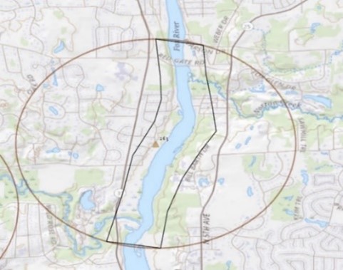
1. An existing stream site location, desired distance and area for stream buffer. Lidar data is also needed for 2 different years.
2. An example would be projects for Illinois_SSRP_Sites_2004_2016 use a standard 1-mile length up and down stream of the site and 100-foot buffer around the 1-mile stream length.
3. These values can be set to any desired length and area for each site. The analysis tools require a length of stream and a buffered area of elevation data to complete the analysis.

Gather data – A few Lidar data retrieval samples

Data will need to be gathered from the most appropriate source for each reach location. The hydrologist requesting the analysis would know potential sources.

Tip

• NOAA Digital Coast Lidar Viewer
• USGS National Map
• USGS Lidar Explorer
• Open Topography
• Various state and university sites, county and local governments, and project specific Lidar collection are other possible sources for data.

Convert Laz to Las (if needed)

1. Add LAStools toolbox to ArcGISPro. Open the LAStools toolbox and select las2lasPro (transform) tool.
2. Drag the folder with the Laz files into the Input folder.
3. Change the output format to Las. Click Run.

Transform LAS file projections

All datasets need to be in the same projection for the entire Study Area.

1. Open LAStools las2lasPro (transform) tool
2. Add the folder for the files that need to be reprojected to the input folder.
3. Chosen projection for transform. Projections must be in feet or meters.

Chose a location to create file storage structure for data.

1. In a folder create a file GDB and a folder labeled LPC. Use the year as the naming convention. Ex. 2025. This is where the LAS Lidar files will go.
2. Create a feature dataset for each GDB. The projection used should be the same as the LAS files for each year. Use site, number, and year for naming convention. Ex. SiteName_120_2025.

Analysis Workflow

Create a Boundary

Boundary within 1 mile buffer

1. Right click on feature dataset and click new Feature Class.
2. Name is boundary and keep feature class type as polygon.
3. Click Finish.
4. Change symbology to black outline.
5. Zoom to your site and create a polygon that surrounds the water system by roughly 100 feet. The distance should be taken from along the entire edge of the stream to account for available elevation data for later analysis.

Create a LAS Dataset

1. In the geoprocessing tab search Create LAS Dataset.
2. In the Input Files select the Folder where the LAS tiles were downloaded to.
3. In the Output LAS Dataset browse to the LPC folder where the two sets of LAS tiles are saved. Name it after the year.
4. Under Surface Constraints the input feature is Boundary.
5. Right click on of the LAS files for the site and go to properties then coordinate system. Copy and paste the coordinate system into the geoprocessing tool.
6. Click run.

See step 9

7. Once tool is finished running, Right click the dataset in the contents pane and select Properties. Under properties click LAS Filter.
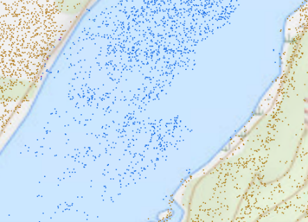
8. Under Classification Codes, make sure only ground, water, and rail are checked. Uncheck all other boxes. Hit Ok.
9. Zoom to the site area to the extent of 1:2000. Make sure you see the classified dots labeled water and ground.

Turn LAS Dataset to Raster

1. In the geoprocessing tab search LAS Dataset to Raster.
2. The Input LAS Dataset will be the one you created in the prior step. Make sure to use the dropdown arrow to select your LAS dataset. Do not drag it from the catalog pane. This will select the LAS dataset with the symbology changes you made prior.
3. The Output Raster location will be the geodatabase you created under the SSRP_Sites folder. Name it DEM_Year. Ex. DEM_2022
4. Value field is Elevation.
5. For Interpolation Type select Binning.
6. Cell Assignment is IDW.
7. Void Fill Method is Natural Neighbor.
8. Output Data Type is Floating Point.
9. For coordinate system in state plane feet: Sampling Type is Cell Size. Change Sampling Value to 1 and Z Factor to 1.
10. Click Run.

Change Symbology of Raster

1. Click on your created raster symbology.
2. Primary symbology should be stretch.
3. Change the color scheme to Elevation #1.
4. Stretch type to Standard Deviation.
5. Statistics to DRA.

Check Raster Pixel Size and columns and rows

1. Zoom into layer at the extent of 1:15.
2. Use the measure tool to measure the length of pixel. Should be 1 ft.
   1. Make sure the measuring tool is set to feet or imperial.
3. Open properties and check that the columns have not been inflated to into the millions.
   1. If there are number of columns in the millions re-run the Las to Raster and set the processing extent to boundary as well and then run again.

Create Cutlines Line Feature Class

1. Right click your geodatabase and click new feature dataset.
2. Keep Output Geodatabase
3. For the Feature Dataset Name, name is Site#_YEAR. Ex. Site263_2008.
4. Use the dropdown box under coordinate system and select the corresponding LAS dataset to select the correct coordinate system.
5. Click Run.
6. Right click the newly created feature dataset and create new feature class.
7. Name it cutlines, Change feature class type to line, and finish.
8. Identify Flow Blockages
   1. Go to the edit ribbon and select create feature and select cutlines
   2. Zoom to the start of the water system and change the extent to around 1:1000.
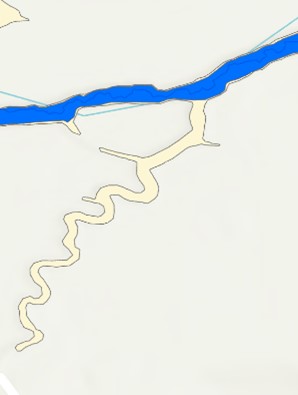
   3. Follow along the water system and look for roads or major crossings that cut off the water system. Draw a line from one end of the waterway to the other side that is cut off. Below are a few examples.

   

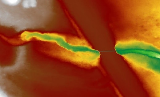
   Cutline example 1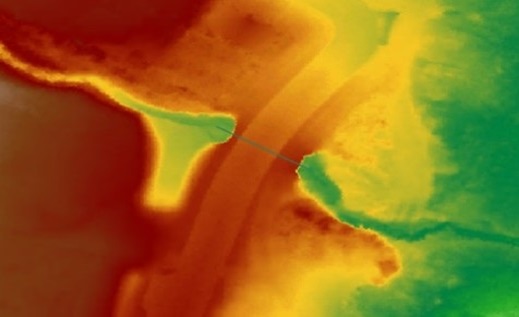

   

   Cutline example 2

9. If there are no blockages create a cutline at each end of the stream.
10. When done, make sure to save edits before doing the next step.

Hydro Modify DEM

1. In the catalog pane, go to the FluvialGeomorph toolbox. Expand tools and select Hydro DEM.
2. For output_workspace, drag your geodatabase from the catalog pane (Created prior) into the space.
3. For cutlines, drag your cutline feature class into the space.
4. For dem, drag your raster dataset into the space.
5. For widen_cells put 4.
6. Click Run.
   1. The result is a DEM without the flow blockages and representing proper water flow across the study area.

Derive Stream as Line Tool – Esri Spatial Analyst Toolbox

1. Open Derive Stream as Line tool
2. Select the dem_hydro as the input surface raster

3. Set the output polyline as stream in the feature dataset.

4. Hit Run. Then repeat for the earlier geodatabase.
5. Change color of streamlines to a bright color to see it better against the dem.
6. Delete all tributaries or lines that are not the main low point flowline. Use split and edit vertices tools. Connect all lines together using the create feature tool.
   1. Make sure the streamline is going through the lowest part of the channel
7. Save edits.

Smooth Line Tool – Esri Cartography Toolbox

1. Set smoothing between 2 and 15 depending on the size and flow of the channel.
2. Check that flowline remains in the channel. Edit flowline or rerun smooth as needed to keep line in channel.

Create Flowline

1. In the FluvialGeomorph toolbox, select the Flowline tool.
2. For the feature_dataset and stream_network drag and drop the corresponding data from the catalog.
3. For smooth_tolerance put 2. It can range from 2-5 based on the range of distribution of the flowline. The goal is to produce a smooth flowline without removing too much resolution from the line.
4. Hit Run Note: Make sure to do most recent data first. Rerun tool for older set of data once done.
5. The output is a line feature class called flowline. This tool derives the site flowline and smooths the stream_network geometry and converts the flowline into a route.
6. Ensure that the flowline remains in the channel and is not simplified into the floodplain. If this occurs, rerun reducing the degree of smoothing.
   1. Also ensure that the red endpoint (vertice) is at the upstream end of the flowline. It is critical that the flowline is digitized in the upstream direction. If this step is not performed, all subsequent tools will malfunction.
7. Open attribute table for each flowline and stream network.
8. The Reach Name must be the same for each flowline and stream network. The name is the Site# and survey event. Ex. Site 264 KANE-DUPAGE County SWCD
9. Check that the flowline is in and near the center of the main channel represented in the ydro_dem.

Create Flowline Points

1. In the FluvialGeomorph toolbox, select the Flowline Points tool.
2. For this tool make sure you do the most recent data first. Find the corresponding data for flowline in the feature dataset.
3. The dem will be the dem_hydro.
4. Km_to_mouth will be 0 in most circumstances.
5. For station_distance put 1. This means there will be a station point for every foot along the flowline.
6. The calibration points, point id field, and measure field will be blank for the most recent data.

7. Leave the search radius default.
8. Hit run.
9. Note: Before you run the flowline points for the older dataset, make sure the newer flowline points tool is done running.
10. For the older dataset, fill in the information like when running the tool for the newer data.
11. For calibration points, drag the flowline points created from the newer data.
12. The point id field is ReachName.
13. Measure field is POINT_M
14. Hit run.
15. The result converts the flowline into a series of points along the reach. The tool converts the flowline feature class into a route, calculates the distance to the mouth of the river for all vertices, and creates a flowline_points feature class.

Create Features

1. Create a new point feature class in either year feature dataset.
2. Add fields for Name (text) and km_to_mouth (double).
3. Drag the ‘features’ feature class into the map. Move it to first in drawing order.
4. Turn off all layers except the flowline points, so you can see the basemap.
5. On the ribbon, click edit and create features.
6. You will create feature at the site # and any other major features on the basemap that the flowline points cross, likes a road, waterway with name, or lake. First, use the explore tool to click on a flowline point. Create the feature on top of the flowline point you selected.
   1. Serve as reference on the profile graph in the report.
7. In the table find the number next to “Measure”. Take note of this number, you will add it to the table once you create the feature.
8. Open attribute table for ‘features’. Under km_to_mouth put the number that was correlated with “Measure”.
9. The name in most cases will just be the name of the street or waterway. For the Site# feature, the name will be Site# and the SSRP_Type found in the attribute table of Illinois_SSRPSites_2004_2016. Ex. Site 264 STP;RR

Reuse the feature layer in future sites

1. Right click on the feature dataset for most recent data. Go to import and select Feature Class(es).
2. For the input features, go to a previous county folder and expand the feature dataset for the most recent geodatabase under any Site# and import that database layer called features.
3. For the output geodatabase, choose the corresponding feature dataset. This allows the use of a layer with existing fields.

REM

1. In the FluvialGeomorph toolbox, select the REM tool.
2. Fill in the parameters with the corresponding data. Make sure for dem you choose the hydro_dem.
3. Buffer distance will be 1500.
4. Hit run. Note: You will not be able to create features and run this tool at the same time.
   1. The purpose of this step is to produce a REM. This DEM normalizes stream bank elevations for a specific reach.
5. Select the symbology for the REM.
6. Change the renderer from Stretch to the Classify.
7. Change number of classes to two.
8. In the first class, change the upper value to 100 and note how the REM changes.
   1. Add onto by this upper value until the dem fills the bank and right before it starts ‘overflowing’ into the floodplain, which is 2 times the depth of the channel.
   2. Get an elevation at the bank and then the center of the channel and add the difference to the 100 first class value.

Find the Channel and Floodplain

1. Have the flowline, demhydro and REM for the newer year.
2. Find the elevation in the REM for the bank and the flowline. Check multiple locations along the stream, including the site location.
3. Find the average difference in elevation between the bank and the flowline.
   
4. Subtract the two REM values to get the bankfull depth for the channel. Ex. bank elevation 104 and flowline elevation 100 then the channel depth is 104. This value is used in the Water Surface Extent tool as the REM_value. This will become the channel bank_raw value.
5. Next Multiply the last number of the channel bank_raw value by 2 and use it as the REM_value for the floodplain bank_raw. Ex. channel bank_raw 104 make the floodplain bank_raw 108.

Create Water Surface Extent

1. In the FluvialGeomorph toolbox, select the Water Surface Extent tool.
2. Fill in the feature dataset and the REM for from the most recent year.
3. Enter the depth value found for the channel
4. Set smoothing to 5.
5. Hit Run
6. Run again for the floodplain depth.

Edit the Channel and Floodplain Banks_raw layers

Sample of a channel bank and floodplain layer

1. Open the attribute table for the channel banks_raw. Sort the Shape_Area column descending.
2. Use the gridcode column value of 1 to find the highest row(s) that make up the stream channel around the flowline. With the channel polygons selected switch the selection and delete all other polygons leaving only the stream channel.
3. The channel banks_raw need to be trimmed of any incoming confluences. Then save the edits.
4. Repeat Create Water Surface Extent for the floodplain banks_raw layer. Leave an additional area or confluences.

Create Cross Sections (only for newest dataset)

1. In the FluvialGeomorph toolbox, select the XS Layout tool.
2. Fill in the feature dataset and flowline from the most recent geodatabase.
3. For split type keep as “split at approximate distance.”
4. Transect spacing is 300.
5. Transect_width is determined by width of floodplain from the flowline. Find the distance of the farthest point of the floodplain from the flowline
6. Transect_width_unit default is used.
7. Hit Run.
   1. The result is a line feature class of regularly spaced cross sections that well represent the channel conditions found in this reach.
   2. Make sure none of the lines are hanging outside the raster area.
8. Select each cross section and make sure green box is on left side of the bank going downstream. Start at upstream going downstream. Make sure the cross sections are parallel to bank. Edit each cross section so that they are perpendicular to the flow of the stream. Adjust their location if they are too close to highways or other smaller streams. The purpose is to get a cross section that extend the full width of the floodplain.
   1. If cross sections cannot be moved without overlapping, they can be deleted. This may occur with tight bends or some meandering of the stream.

XS Resequence (only for the newest dataset)

1. Run only if any cross sections were deleted in the adjustment process.

Calculate Cross Section Watershed Area (only for newest dataset)

1. In the fluvialgeomorph folder, expand layers and add NHDPlusFac_National.tif
2. Right click the layer, go to data, then export raster
3. Add the output to whatever year folder.
4. Clipping geometry is displaying current extent. Make sure you are zoomed out to the whole county, so each site is located within extent.
   1. Optional: Create a clip for each project site of the NHDPlusFac_National.tif with the extent zoomed out 1:50000 centered on the site.
5. Go to FluvialGeomorph toolbox. Add Wastershed Area tool.
6. Snap distance is 100.
7. Start with the more recent data first.
8. Hit Run.
   1. If it doesn’t work zoom into the mile radius of site and clip FAC. Having a smaller clip will also reduce the tool runtime.
   2. The result is a new attribute field in the XS feature class that has a calculated watershed area for each regularly spaced cross section.
9. Once it is done running, open attribute table and see if anything in the watershedareaSqMile is off.
   1. Some of the cross sections Watershed_Area_SqMile may not follow the trend. If this is the case, manually enter in the values to fill in the gaps. If most of the cross sections are missing these or display incorrect values, rerun Watershed Area tool and increase the snap distance.
   2. Check for other streams and bodies of water feeding into the stream that would validate the abrupt changes in the watershed area.
10. Import the finished xs_300_100 to the earlier year feature dataset.

XS River Position

1. In the FluvialGeomorph toolbox, select XS River Position.
2. Enter feature dataset for more recent geodatabase.
3. Input Cross Sections.
4. Input Flowline Points.
5. Hit Run.
6. The result adds new fields in the attribute table of the XS feature class.
7. Two temporary charts will populate the Contents tab under the Cross Section Line Feature Class (XS Seq by km_to_mouth, XS Seq by Watershed Area sq mile). If the charts are removed from the contents pane, you will need to run the XS River Position Tool to view them again.
   1. Open both Charts and inspect for any issues in the data.
   2. Note: This step provides charts which help see if there are gaps in the data.
8. Repeat XS River Position for the older gdb.

XS Points

1. In the FluvialGeomorph toolbox, select XS Points.
2. Enter feature dataset for more recent geodatabase.
3. Input Cross Sections.
4. Input dem_hydro.
5. Change dem_units to ft.
6. Input REM for the REM_dem.
7. Station Distance is 1.
8. Hit Run.
9. Points have been created every foot along the Cross Section with an Elevation. This will provide a visual elevation profile for each cross section.
10. Repeat these steps for the older gdb.

XS Point Classify

1. In the FluvialGeomorph toolbox, select XS Points Classify.
2. Enter feature dataset for the most recent year.
3. Input XS points.
4. Input channel polygon.
5. Input floodplain polygon.
6. Leave buffer distance default.
7. Repeat for earlier year XS Points.

Run Report

XS Dimensions Level 1

1. In the FluvialGeomorph toolbox, open XS Dimensions, Level 1.
2. XS’s are added into xs_line fc.
3. Enter 4 for the lead_n.
   1. This sets the moving window to average 4 XS’s above and below the XS being calculated.
4. Leave the use_smoothing box unchecked and loess_span as 0.1.
5. Check that the vert_units are in ft.
6. After the tool completes, refresh the folder the gdb is in and you should find a .csv file in there.

Join from CSV (Data Management toolbox)

1. In the FluvialGeomorph toolbox, open Join From CSV located in the Data Management toolset.
2. Feature_dataset will be the feature dataset of the most recent gdb.
3. Fc will be the XS line feature class.
4. Choose Seq in the dropdown for the fc_field.
5. The csv_file will be the .csv file created from the XS Dimensions Level 1 Tool.
6. Csv_field will match the fc_field so it should also be Seq.
7. Hit Run.
8. A new line feature class ending with dims_L1 will be added to the feature dataset.

Generate Level 1 Report

1. In the FluvialGeomorph toolbox, open the Report – L1 located in the Reports toolset.
2. Stream will be the ReachName which was created when making the flowline. Copy and paste the ReachName from XS’s attribute table.
3. Flowline_fc will be the flowline feature class from the recent year.
4. Xs_dimensions_fc will be the line feature class created during the Join From CSV tool.
5. Flowline_points_1 will be the flowline points from the most recent year.
   1. Flowline_points_2 will be the flowline points from the older year.
6. Xs_points_1 will be the XS points point feature class created from the XS Points tool. Use the data from the most recent year.
   1. Xs_points_2 will be the XS points point feature class for the older year.
7. Survey_name_1 will be the year of the most recent data (ex: 2022).
   1. Survey_name_2 will be the year of the older data (ex: 2012).
8. Features_fc will need the features point feature class that was created to indicate roadways, site improvements, or other bodies of water.
9. Channel_fc will be the lower number bank_raw layer that represents the channel.
10. Floodplain_fc will be the higher number bank_raw layer that represents the floodplain,
11. Dem will need the dem_hydro.
12. Check the box for: show_xs_map.
13. Change profile_units to feet.
14. Check boxes for aerial and elevation.
15. Xs_label_freq and exaggeration should already be set to 10 and extent_factor is 1.2.
16. Output_dir is where the report will be stored. Each project has a Reports folder.
17. Output_format is word_document.
18. Hit Run.
19. Review report for errors and anomalies in the data.