11  Level-3 Planform Analysis

🔴 Advanced

The purpose of this SOP is to demonstrate the workflow of fluvial geomorphology (fluvgeo) rapid watershed assessment in ArcGIS Pro. This approach uses a suite of planning analysis tools to rapidly assess and identify sediment sources, pathways, and sinks for watershed analysis. Level 1 is to extract basic channel dimensions. This stage develops terrain, defines the stream reach, creates cross sections and identifies features along the reach. The output is a report of the dimensions for each cross section on a reach.

Application and Data Setup

🔧 Practical

Applications

Level-2 Data

1. Sites must have had up through Level-2 analysis run. That data is essential to completing Level_3 analysis.
2. Software application and tools from Level-1 will be needed for Level-3 analysis.

Data access in ArcGIS Pro

1. Fluvgeo toolbox requires the use of a mapped drive for accessing the data in ArcGIS Pro. UNC connection will create errors with some of the Fluvgeo tools.
2. Create a mapped drive and use that connection in ArcCatalog.

Analysis Workflow

🔧 Practical

Define Valley Line

Develop Candidate Valleylines

The following steps are performed in the site geodatabase for the base year. This is done to ensure that a valleyline feature class is created smoothly through all of the reaches in a site.

1. Use the flowline to determine the valley line for the reach.
2. Open the ESRI 🛠️ Smooth Line tool to smooth the reach 🗺️ flowline feature class from the most recent year as the input feature.
3. For the first candidate valleyline, use a 📊 Smoothing Tolarance value of 🧮 200 meters. In this case you would name the output feature class valleyline_200 and put in the same feature dataset.

NoteWhat Smoothing Tolerance Value?

It depends! See Tech Manual for discussion on determining planform scale.

4. Choose the 🧮 PAEK smoothing algorithm.
5. Set the 📊 smooth tolerance to 🧮 200
6. Click Run.
   1. Repeat the previous step using the 📊 Smoothing Tolerance values such as 🧮 400, 🧮 800, and 🧮 1000.
   2. Depending on the detail of the 🗺️ flowline feature class geometry, you may need to select a different range or set of step values of the 📊 Smoothing Tolerance parameter values to evaluate.
7. The goal is to create a wide degree of flowline smoothing in the candidate valleyline feature classes to select from in the next step.
8. Choose Final 🗺️ Valleyline feature class.
9. Add the 🗺️ floodplain polygon (higher bank_raw_###) and all of the candidate 🗺️ valleyline feature classes to the current map.
10. Identify the 🗺️ valleyline feature class that has the highest smoothing tolerance value that also is mostly contained within the extent of the 🗺️ floodplain polygon feature class.

Valleyline Buffer

The valleyline should be considered a fuzzy area representing the center of the valley.

1. Add the 🗺️ valleyline feature class as the input.
2. Add the output multi-ring buffer to the newest year gdb. Name it 🗺️ multiring_buffer feature class.
3. Use the identifies valleyline to create a multi-ring buffer. Use the the distance at a narrow part of the reach as the first buffer distance. The following increments can be set 5, 10, or desired distances. Create 3 to 5 rings.
4. Leave the remaining settings as the defaults.
5. Hit Run.
6. Add the bankline layer to the map.
7. Identify the buffer ring that best shows the baklines looping out of the buffer ring from side to side. The chosen ring should show the loops at a smaller scale.

NoteScale and distance to use to define valleyline buffers!

It depends on your reach! See Tech Manual for discussion on determining planform scale.

8. Select and export the chosen buffer ring as new layer in the gdb.
9. In the site geodatabase of the base year, rename the selected buffer ring to distance_buffer_year. Ex. 20ft_buffer_2012
10. Delete the multi-ring buffer feature classes from the site geodatabase of the base year.
11. Copy the selected distance buffer feature class you just created from the site geodatabase to each of the base year reach geodatabases.

Define Meander Loops

The stage defines meander loops and bends for the base year for each reach.

Define Loop Points Layer

1. Create a new point feature class named 🗺️ loop_points feature class. 📊 Enable 🧮 z and m values. The feature class should contain the following fields:
   1. 📊 ReachName: 🧮 Text (50) - The purpose of this field is to store the reach name.
   2. 📊 loop: 🧮 Long Integer - The purpose of this field is to store the loop unique identifier for the point.
   3. 📊 bend: 🧮 Long Integer - The purpose of the field is to store the bend identifier for the point.
   4. 📊 position: 🧮 Text (10) - The purpose of this field is to store position identifier for the point. This field must have one three values: 🧮start, 🧮end, or 🧮apex.

Create Loop Points

NoteHow to Identify Loops.

1. 🗺️ Loop_points features are used to define the start and end location of loop bends and the location of a loop’s apex.
2. 🗺️ Loop_points features are always placed along (i.e., snapped to) an outer bankline of the feature.

1. Begin numbering loops starting at the downstream end of the reach and increment the loop integer values moving upstream.
2. Beginning and end of loops are delineated where the valleyline definitively crosses the flowline.

Step 2

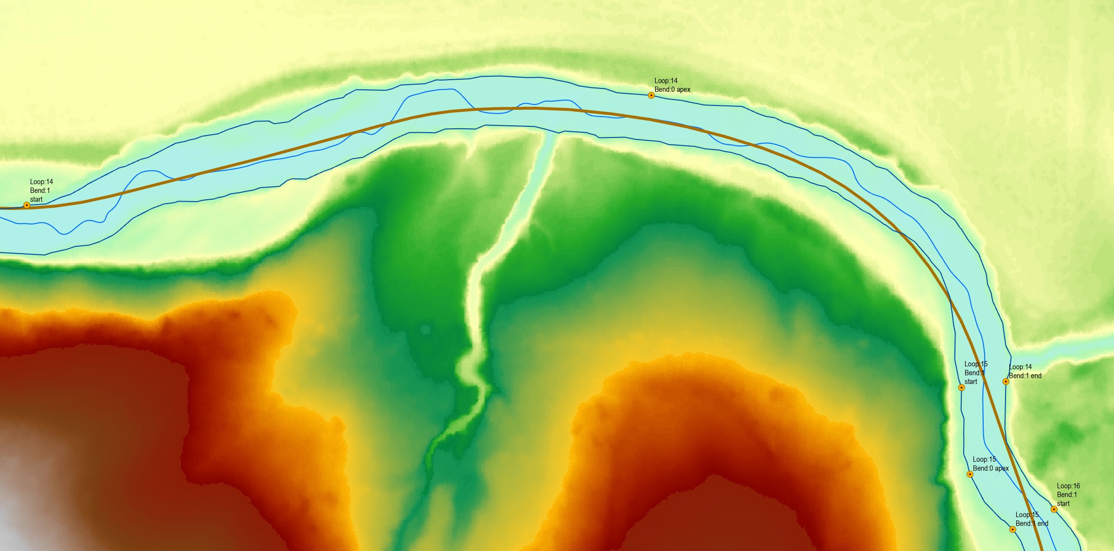
3. If the flowline crosses the valleyline and then crosses back over in a short distance, this is not considered a definitive crossing. A definitive crossing is one where the flowline approaches the valleyline, crosses it, and then continues to move away from the valleyline for a significant longitudinal distance.
4. Loops must alternate from one bank to the opposite bank. For example, if loop 1 is delineated along the right descending bank, then loop 2 is delineated along the left descending bank.
5. Loops are composed of one or more bends (bends nest inside of loops). For example, loop 1 can have bends 1, 2, and 3 (i.e., loop 1, bend 1; loop 1, bend 2; loop 1, bend 3).
6. Bend numbering restarts within each loop. The first bend value within a loop always begins with the value 1.
7. Create start, end, and apex points (complete all attribute information).
8. Save Edits.

NoteMultiple Reaches:

• For a site with multiple reaches, loops must be uniquely numbered across all reaches. The loop field values of loop_points should not repeat within the reaches of a site.
• The downstream-most loop in the site should be numbered starting with the loop field value of 1 and increase moving upstream.
• Set the loop field value for each upstream reach to the upstream-most value (i.e., the highest loop value of the downstream reach’s 🗺️ loop_points feature class) of the downstream reach. For example, set the value of the field loop of the first Reach-2 loop_points feature to 8 if the maximum value of Reach-1’s loop_points feature class loop field is 7.

Check Loop Points:

• Use the 🛠️ Check Loop Points tool in the 🧰 Check toolset to verify that loops and bends are defined correctly.
• Review the messages produced by this tool to identify and correct problems with loop and bend delineation.

Derive Bankline Points

The purpose of this step is to convert the banklines to a set of bankline_points and assign elevations and loop and bend locations to these features.

1. Open the 🛠️ Bankline Points tool to assign loops, bends, elevations and valley line positions to the 🗺️ bankline_points feature class.
2. Add the feature dataset for the most recent year.
3. Add the 🗺️ loop point, 🗺️ banklines, and 🗺️ valleyline feature classes from the most recent year.
4. Add the 🗺️ demhydro raster for the mosts recent year.
5. Set the 📊 station_distance at 🧮 1.
6. Hit Run.
7. In the 🧰 Check toolset run the 🛠️ Check Bankline Points tool.
   1. The check tool ensures that the 📊 loop, 📊 bend, 📊 position, 📊 valley_POINT_X, 📊 valley_POINT_Y, and 📊 valley_POINT_M fields are populated. Only bankline_points features within loops and bends will have values in the 📊 loop, 📊 bend, and📊 position` fields.
   2. All records should have values in the 📊 valley_POINT_X, 📊 valley_POINT_Y, and 📊 valley_POINT_M fields.
8. Apply the following definition query to the 🗺️ bankline_points feature class: “loop IS NOT NULL”. Only bankline_points features between loop_points features should be visible.

Assign Cross Section Loops

The purpose of this step is to assign loop and bend identifiers to regularly spaced and riffle cross section feature classes for each reach.

1. Open the 🛠️ Assign Loops tool to assign loops and bends to a 🗺️ XS line feature class.
2. Add the 🗺️ cross_section feature class from the the most recent survey event dataset.
3. Add the 🗺️ bankline_points feature class to the most recent survey event dataset
4. Once the tool completes check the regular cross section feature class attribute table correctly assigned the loop and bend field values.
5. Repeat this step for both the 🗺️ riffle_channel and 🗺️riffle_floodplain feature classes.

Run Report

🔧 Practical

XS Dimensions Level 3

The purpose of this stage is to calculate the Level 3 dimensions for each reach.

Calculate Cross Section L3 Dimensions

The purpose of this step is to calculate the L3 dimensions for the regularly spaced and 🗺️ riffle _XS feature classes for each reach.

Note

If any 🗺️ *_dims_L3 feature classes exist in the reach geodatabase (created during a previous run), delete these feature classes.

1. Open the 🛠️ XS Planform, Level 3 tool to calculate the L3 dimensions.
2. Add the 🗺️ level 2 XS_Dimensions feature class from the same survey event to 🗺️ xs_dimesions.
3. Add the 🗺️ bankline_points feature class from the same survey event to 🗺️ bankline_points feature class.
4. Refresh the Survey event year folder to update with the 📈 XS-Planform Level 3 csv.
5. Verify in the attribute table that the L3 dimensions have been calculated

Join from CSV (Data Management toolbox)

1. Open the 🛠️ Join from CSV tool in the 🧰 Data Management toolbox.
2. Add the feature dataset for the current survey event.
3. Add the 🗺️ level 2 XS_Dimensions feature class from the same survey event to 📊 fc.
4. Select the 🧮 Seq in the dropdown for the 📊 fc_field.
5. Add the 📈 level 3 dimension csv spreadsheet to the 📊 csv_file.
6. Type 🧮 Seq into the 📊 csv_field.
7. Hit Run.
8. Verify in the attribute table joined of the L3 dimensions csv have been added.

Add Modeled Water Surface Elevation (Optional)

1. Open the 🛠️ RAS Watersurface tool.
2. Add the feature dataset for the current survey event.
3. Add the 🗺️ xs_dimensions_l3 feature class to 📊 xs_dims.
4. Add a 🗺️ ras HEC model raster containing water surface elevation field.
5. Name the model ouput (Use the RAS_model_name parameter to distinguish between multiple RAS model scenarios)

Generate Level 3 Report

The purpose of this stage is to run the Level 3 report for each reach.

1. Open the 🛠️ Level 3 Report tool to produce the Level 3 Report.
2. Add the value of the 📊 ReachName field used in the 🗺️ flowline feature class to 📊 stream.
3. Add the 🗺️ flowline feature class for the base year survey to 📊 flowline_fc.
4. Add the 🗺️ XS line feature class to 📊 xs_fc.
5. Add the 🗺️ *_dims_L3 feature class calculated for the regular cross sections of the most recent survey event.
6. Add the 🗺️ xs_points_* feature class for the most recent survey event first (i.e., the base year) and then the previous surveys in reverse chronological order (e.g., 2016, 2010, 2006).
7. Enter the most recent survey event first and then the the previous surveys in reverse chronological order (e.g., 2016, 2010, 2006).
8. Add the 🗺️ DEM raster for the most recent survey event.
9. Add the 🗺️ banklines feature class created for the most recent survey event.
10. Add the 🗺️ features point feature class for the site to the 📊 features_fc.
11. Enter the same 🧮 bf_estimate from level 2 report into the 📊 bf_estimate box.
12. Enter the same regions used in level 2 report or as others as needed.
13. Check show map box.
14. Set the profile units to the units of the surface raster.
15. Leave 🧮 aerial and 🧮 elevation boxes 📊 checked.
16. Leave the 🧮 defaults for 📊 xs_label_freq, 📊 exaggeration, and 📊 extent_factor.
17. Select the folder that the report should be written to.
18. Select 🧮 word as the 📊 output format for the report.
19. Hit Run.

Next Steps

☑️ Evaluate

Review the report.

1. Go to chapter Level 3 Planform Report under Report Reviews.
2. Refer to the FG Technical Manual as need for more detailed information.
3. Revise and/or rerun as needed.