9  Level-2-EB Estimate Bankfull Analysis

🟡 Intermediate

The purpose of this SOP is to demonstrate the workflow of fluvial geomorphology (fluvgeo) rapid watershed assessment in ArcGIS Pro. This approach uses a suite of planning analysis tools to rapidly assess and identify sediment sources, pathways, and sinks for watershed analysis. Level 2 is to estimate the REMed bankfull elevation for the base year for each reach. This is accomplished by identifying and mapping of all cross sections and roughly estimate channel bankfull dimensions and profile for each reach. The data from level 1 will be needed to start the level 2 process. This analysis begins with modifications to the cross sections.

Application and Data Setup

🔧 Practical

Applications

1. ArcGIS Pro mapping application with adequate system privileges ArcGIS Pro w/Admin Privileges to install and update toolsets.
2. R, Rstudio and Rtools to run the Fluvgeo tools in ArcGIS Pro.

Retreive the most current version of FluvGeo Toolbox from GITHUB

1. Get the latest version of the toolbox from this page under Releases.https://github.com/FluvialGeomorph/FluvialGeomorph-toolbox
2. Place the install in a location that all required applications can access.
3. In Rstudio under tools install package HERE.
4. In ArcCatalog open the 🧰 Fluvgeo toolbox and under install click Install R Package box and Hit run.

Data access in ArcGIS Pro

1. 🧰 Fluvgeo toolbox requires the use of a mapped drive for accessing the data in ArcGIS Pro. CNC connection will create errors with some of the Fluvgeo tools.
2. Create a mapped drive and use that connection in ArcCatalog.

Analysis Workflow

🔧 Practical

Create Feature Class

1. Copy the most recent years cross section 🗺️ XS as line feature class named 🗺️ riffle_floodplain feature class.
   1. You’ll use the original XS lines that represent the rock riffles and delete all others.
   2. extend each XS line high ground to high ground of the dem_hydro outside the floodplain on each side. XS extent must be beyond the floodplain at minimum and kept perpendicular to the channel.
   3. This provides a feature class already with correct projection and attribute fields.

Identify Rock Riffles

Riffle Identifying Characteristics:

• A straight reach between two meander bends, areas in the cross-overs between river bends
• Clear indicators of the active floodplain or bankfull discharge
• Presence of one or more terraces
• Channel section and form typical of the stream
• A reasonably clear view of of geomorphic features
• Areas of high water surface slope (in the case of high gradient streams)
• Areas of minimum depth and width
• Channel width parallel and consistent
• Avoid tributary influences
• Cross sections should be drawn wide enough to capture the top of bank

Digitize Riffles

1. Digitize riffle cross sections beginning with the left descending bank. While editing, use the Reverse Direction command (aka flip) to ensure riffles are digitized in the correct direction.
   1. A red vertex denotes the end of a line segment. Therefore, the red end vertex should be on the right descending bank.
   2. Check that each cross section is digitized in the correct direction (start at the left descending bank and end on the right descending bank) before going on to the next step.
   3. Ensure that riffle cross sections are digitized to the full width of the active floodplain. Edit each feature to ensure that it extends at least to the edge of the floodplain boundary layer, but no further.

Note

For a site with multiple reaches, riffle cross sections must be uniquely numbered across all reaches. The 📊 Seq field values of riffle cross sections should not repeat within the reaches of a site.

2. The downstream-most cross section in the site should be numbered starting with the Seq field value of 1 and increase moving upstream.
   1. If necessary, use the tool to set the starting 📊 Seq value for each reach.

Calculate Cross Section Watershed Area

1. Go to FluvialGeomorph toolbox open the 🛠️XS Wastershed Area tool.
2. Start with the more recent data first.
3. Add the 🗺️ features point feature class.
4. Add the extended 🗺️ XS line feature class.
5. Add the 🗺️ flowline feature class.
6. Add the 📊 flow_accum created in level or refer to level 1 instructions.
7. 📊 Snap distance is 🧮 100.
8. Hit Run.
   1. If it doesn’t work zoom into the mile radius of site and clip FAC. Having a smaller clip will also reduce the tool runtime.
   2. The result is a new attribute field in the 🗺️ XS line feature class that has a calculated watershed area for each regularly spaced cross section.
9. Once it is done running, open attribute table and see if anything in the 📊 watershedareaSqMile is off.
   1. Some of the cross sections 📊 Watershed_Area_SqMile may not follow the trend. If this is the case, manually enter in the values to fill in the gaps. If most of the cross sections are missing these or display incorrect values, rerun the Watershed area tool and increase the snap distance.
   2. Check for other streams and bodies of water feeding into the stream that would validate the abrupt changes in the watershed area.
10. Run for older geodatabase.

XS River Position

1. In the FluvialGeomorph toolbox, select 🛠️ XS River Position.
2. Enter 🗺️ features point feature class for more recent geodatabase.
3. Input extended 🗺️ XS line feature class.
4. Input 🗺️ flowlinepoints feature class.
5. Hit Run. Complete for both the 🗺️ channel_XS and 🗺️ floodplain_XS feature classes.
6. The result adds new fields in the attribute table of the 🗺️ XSline feature class.
7. Two temporary charts will populate the Contents tab under the 🗺️ XS line feature class (📊 XS Seq by 📊 km_to_mouth, 📊 XS Seq by 📊 Watershed Area sq mile). If the charts are removed from the contents pane, you will need to run the 🛠️ XS River Position Tool to view them again.
   1. Open both Charts and inspect for any issues in the data.
   2. Note: This step provides charts which help see if there are gaps in the data.
8. Repeat 🛠️ XS River Position for the older gdb.

XS Points

1. In the FluvialGeomorph toolbox, select 🛠️ XSpoints.
2. Enter 🗺️ features point feature class for more recent geodatabase.
3. Input extended 🗺️ XS line feature class.
4. Input 🗺️ dem_hydro raster.
5. Change 📊 dem_units to 🧮 ft.
6. Input 🗺️ REM raster for the REM_dem.
7. 📊 Station Distance is 🧮 1.
8. Hit Run. Complete for both the 🗺️ channel_XS and 🗺️ floodplain_XS point feature classes.
9. Points have been created every foot along the Cross Section with an Elevation. This will provide a visual elevation profile for each cross section.
10. Repeat these steps for the older gdb.

XS Point Classify

1. In the FluvialGeomorph toolbox, select 🛠️ XS Points Classify.
2. Enter 🗺️ features point feature class for the most recent year.
3. Input extended 🗺️ XSpoints feature class.
4. Input 🗺️ channel polygon feature class.
5. Input 🗺️ floodplain polygon feature class.
6. Leave 📊 buffer distance as the 🧮 default.
7. Repeat for earlier year extended 🗺️ XSpoints feature class.

Create Banklines

1. Turn 🗺️ channel bank_raw polygon feature class into a line layer.
2. Use Esri 🛠️ Poygon to Line tool.
3. Add the 🗺️ bank_raw channel polygon feature class as the input feature.
4. Add the 🗺️ features point feature class for the more recent gdb.
5. Hit Run.

Edit channel line layer

Step 2

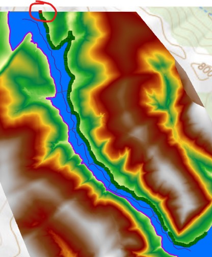
1. Split the line and remove all parts that are not the streambank length of the flowline.
   
2. Set the flow on each streambank line to flow downstream. (Make sure the RED node is at the upstream end of the line and both ends are snapped together)
   
3. Save edits.

XS Dimensions Level 1

1. In the FluvialGeomorph toolbox, open 🛠️ XS Dimensions, Level 1.
2. Extended 🗺️ XS line feature class for the newest year are added into xs_line fc.
3. Enter 🧮 4 for the 📊 lead_n.
   1. This sets the moving window to average 4 XS’s above and below the XS being calculated.
4. Leave the 📊 use_smoothing box 🧮 unchecked and 📊 loess_span as 🧮 0.1.
5. Check that the vert_units are in ft.
6. After the tool completes, refresh the folder the gdb is in and you should find a .csv file in there.

Join from CSV (Data Management toolbox)

1. In the FluvialGeomorph toolbox, open 🛠️ Join From CSV located in the Data Management toolset.
2. 🗺️ features point feature class will be the feature dataset of the most recent gdb.
3. Fc will be the 🗺️ XS line feature class.
4. Choose 🧮 Seq in the dropdown for the 📊 fc_field.
5. The csv_file will be the .csv file created from the 🛠️ XS Dimensions Level 1 Tool.
6. 📊 Csv_field will match the 📊 fc_field so it should also be 🧮 Seq.
7. Hit Run.
8. A new line feature class ending with 🗺️ *dims_L1 will be added to the feature dataset.

Go to the USGS StreamStats website

Get the 50-percent AEP flood value for the stream reach.

Note

Other sources can be used to get the watershed discharge. 
Check with hydrologist requesting the analysis for additional sources.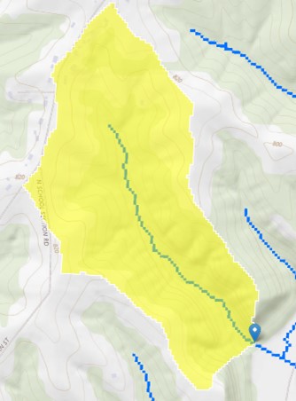

Step 3. i

1. Select the state of the reach on the left of the stream.
2. Zoom into the location for the stream reach until the stream layer shows.
3. Click the delineate button.
   1. On the map select the base of the stream reach. The watershed calculation will start. When it is complete a delineation of the reach will show.
   2. Click Continue.
   3. Select all 4 options under Regression Based Scenarios.
   4. Below expand Basin Characteristics and Select All Basin Characteristics.
   5. Click Continue. The calculations for the report will run.
   6. Once the calculations are completed scroll to the bottom of the left panel, check all the boxes and click Open Report.
   7. Add the site name to the report title. a. Ex. Site193 JODAVIESS County SWCD Stream Stats Report.
   8. Add any comments need to the comment section.
   9. Scroll to the bottom and print the report to PDF. Save to the 📁 site folder.

Open the PDF Stream Stats Report

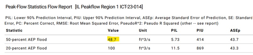
1. Locate the 50-percent AEP flood value under the Peak-Flow Statistics Flow Report section around page 8 of the report. This value will be used in the Level 2 report.

Run Report

🔧 Practical

L2 XS Dimensions

1. In the FluvialGeomorph toolbox, open 🛠️ XS Dimensions, Level 2.
2. 🗺️ XS dimension level 1 line feature class for the riffles into extended 📊 xs_line fc.
3. 🗺️ XSpoints feature class for the channel riffles are added to the extended 📊 XS_point_fc.
4. Bankfull_elevation is from the channel depth of the 🗺️ bank_raw_channel feature class. Ex. 103.5
5. Enter 4 for the 📊 lead_n.
   1. This sets the moving window to average 4 XS’s above and below the XS being calculated.
6. Leave the 📊 use_smoothing box 🧮 unchecked and 📊 loess_span as 🧮 0.1. Can be adjusted up to 1.
7. Check that the 📊 vert_units are in 🧮 ft.
8. 📊 Discharge method is🧮 model_measure`.
9. 📊 Discharge_value is the 50-percent AEP flood value from the watershed discharge report.
10. After the tool completes, refresh the folder the gdb is in and you should find a .csv file in there.

Join from CSV

1. In the FluvialGeomorph toolbox, open 🛠️ Join From CSV located in the 🧰 Data Management toolset.
2. Feature_dataset will be the 🗺️ features point feature class of the most recent gdb.
3. Fc will be the extended 🗺️ XS_layout_dims_L1 line feature class.
4. Choose 🧮 Seq in the dropdown for the 📊 fc_field.
5. The csv_file will be the 📈 .csv spreadsheet file created from the 🛠️ XS Dimensions Level 2 Tool.
6. 📊 Csv_field will match the 📊 fc_field so it should also be 🧮 Seq.
7. Hit Run.
8. A new line feature class ending with 🗺️ *dims_L2 line feature class will be added to the feature dataset.

Generate Level 2 Report

1. In the FluvialGeomorph toolbox, open the 🛠️ Report – L2 located in the 🧰 Reports toolset.
2. 📊 Stream will be the 🧮 ReachName which was created when making the flowline. Copy and paste the ReachName from XS’s attribute table.
3. 📊 Flowline_fc will be the 🗺️ flowline feature class from the recent survey event.
4. 📊 Extended Xs_fc will be the 🗺️ XS line feature class for the most recent survey event.
5. 📊 Extended Xs_dimensions_fc will be the line feature class created during the 🛠️ Join From CSV tool.
6. 📊 Extended Xs_points_1 will be the 🗺️ XSpoints feature class created from the XS Points tool. Use the data from the most recent survey event.
   1. Extended Xs_points_2 will be the 🗺️ XSpoints feature class for the older event.
7. 📊 Survey_name_1 will be the survey event of the most recent data (ex: 2022).
   1. 📊 Survey_name_2 will be the survey event of the older data (ex: 2012).
8. 📊 Features_fc will need the 🗺️ features point feature class that was created to indicate roadways, site improvements, or other bodies of water.
9. 📊 Channel_fc will be the lower number bank_raw layer that represents the channel.
10. 📊 Floodplain_fc will be the higher number bank_raw layer that represents the floodplain,
11. 📊 Dem will need the 🗺️ dem_hydro raster from the most recent survey event.
12. 📊 Bf_estimate will be the 🧮 50-percent AEP flood from Stream Stats or other source.
13. Regions will be selected based on needs for the site. They calculate an estimate of specific hydraulic dimension for a given drainage area. One to four curves can be selected for a report. Ex. IL sites normally use Southern Driftless, Lower Southern Driftless, and Eastern United States.
14. Check the box for: 🧮 show_xs_map.
15. Change 📊 profile_units to 🧮 feet.
16. Check boxes for 🧮 aerial and 🧮 elevation.
17. 📊 Xs_label_freq and 📊 exaggeration should already be set to 🧮 10 and 📊 extent_factor is 🧮 1.2.
18. 📊 Output_dir is where the report will be stored. Each project has a Reports folder.
19. 📊 Output_format is 🧮 word_document.
20. Hit Run.
21. Review report for errors and anomalies in the data.

Next Steps

☑️ Evaluate

Review the report.

1. Go to chapter Level 2 Estimate Bankfull Report under Report Reviews.
2. Refer to the FG Technical Manual as need for more detailed information.
3. Revise and/or rerun as needed.